Variational Autoencoders (VAEs)

TL;DR

• What is a VAE? A Variational Autoencoder (VAE) is a generative model that learns to create new data by compressing inputs into a probabilistic latent space and then decoding them.
• Core Architecture: It consists of an encoder that maps an input to a probability distribution (mean and variance) in the latent space, and a decoder that reconstructs the input from a sample of that distribution.
• Training Objective (ELBO): VAEs are trained by balancing two objectives: a reconstruction loss that ensures the generated data resembles the original, and a KL divergence loss that organizes the latent space into a smooth, continuous structure.
• Key Innovation: The reparameterization trick makes the sampling process differentiable, allowing the entire model to be trained with standard backpropagation.
• Limitations & Modern Use: While early VAEs often produced blurry images, their architecture is foundational to modern AI. In models like Stable Diffusion, a VAE acts as a powerful "perceptual codec," compressing images into a manageable latent space where the diffusion process can run efficiently.

Variational Autoencoders (VAEs) are a powerful type of generative models that combine the principles of autoencoders with variational inference. They are particularly effective for generating new data samples that resemble the training data, while also providing a structured latent space.

Unlike a standard autoencoder designed for simple compression, a VAE's latent space is smooth and meaningful. This structure allows you to sample a random point and decode it into a novel, coherent output, making VAEs a cornerstone of generative AI.

How Does a VAE Work? The Encoder-Decoder Architecture

---

A standard autoencoder compresses an input $x$ (like an image) into a single, deterministic point $z$ in a latent space, and a decoder tries to reconstruct $x$ from $z$. This is good for compression, but the latent space is often "brittle" and disorganized, with gaps between encodings. You can't just pick a random point and expect it to decode into something meaningful.

A VAE solves this by making the bottleneck probabilistic. The architecture consists of two main parts: an encoder and a decoder

Diagram of a Variational Autoencoder architecture, showing the encoder, probabilistic latent space, reparameterization trick, and decoder

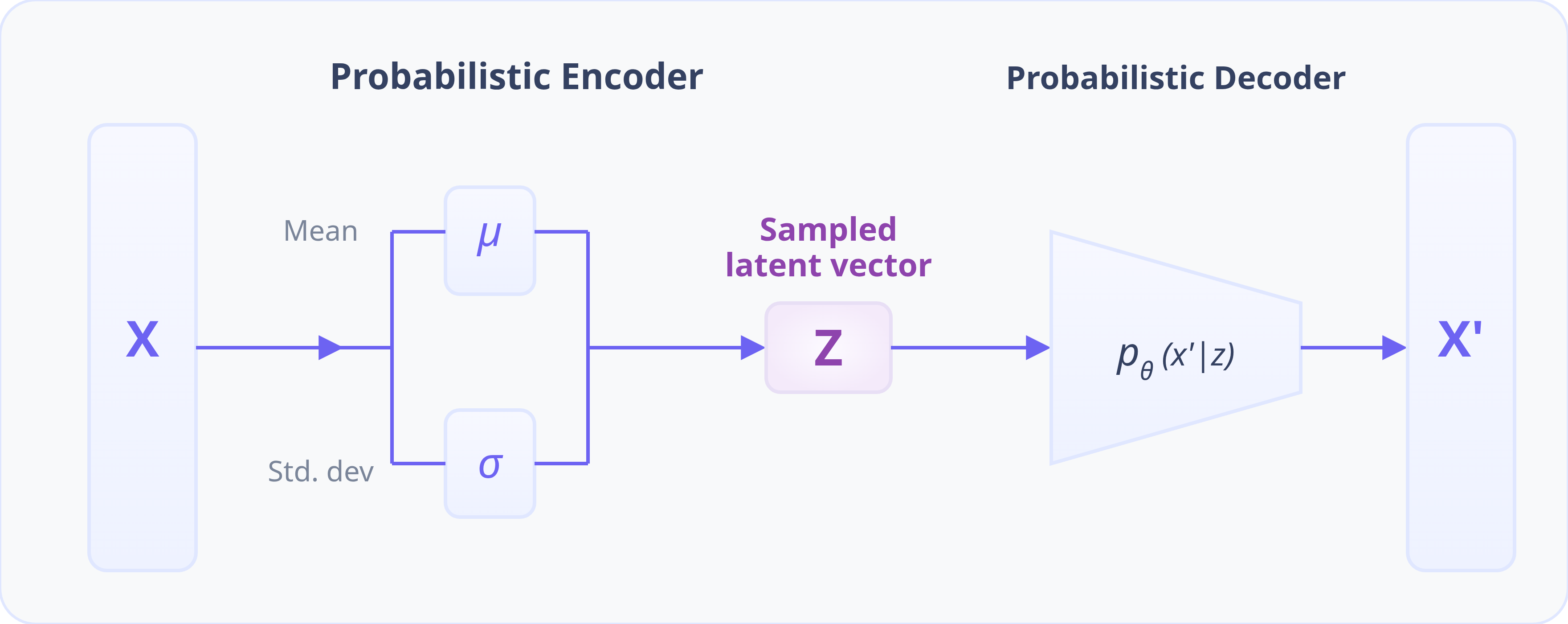
The Encoder: Mapping Inputs to a Probabilistic Latent Space

The first step is the encoder $q_\phi(z|x)$. Instead of mapping an input $x$ to a single point $z$, the encoder maps it to a distribution over the latent space. Specifically, it outputs the parameters of a simple Gaussian distribution: a mean vector $\mu$ and a variance vector $\sigma^2$. This distribution represents our "probabilistic cloud," or belief about where the most suitable latent code $z$ for the input image $x$ should lie.

The Reparameterization Trick: Making Sampling Differentiable

Next, we need to get a latent vector $z$ by sampling from the distribution $N(\mu, \sigma^2)$ predicted by the encoder. However, the sampling operation is random and non-differentiable, which would prevent gradients from flowing back to the encoder during training.

The reparameterization trick elegantly solves this. We redefine the sampling of $z$ as:

$$z = \mu + \sigma \cdot \epsilon$$

Here, $\epsilon$ is a random sample drawn from a fixed standard normal distribution $N(0, I)$. This formulation isolates the randomness as an external input. The network still produces the deterministic parameters $\mu$ and $\sigma$, allowing gradients to flow through them unimpeded. This makes the entire VAE trainable with standard backpropagation.

A note on implementation: For numerical stability, the encoder network typically outputs the logarithm of the variance, $\log(\sigma^2)$. We can then calculate the standard deviation as $\sigma = \exp(0.5 \cdot \log(\sigma^2))$, which ensures $\sigma$ is always positive. To generate a latent vector $z$, we need to sample from the distribution $N(\mu, \sigma^2)$ predicted by the encoder. However, the sampling operation itself is random and non-differentiable, which breaks the backpropagation needed for training.

The Decoder: Reconstructing Data from the Latent Space

Finally, the sampled latent vector $z$ is passed to the decoder $p_\theta(x|z)$. The decoder's job is to take this latent code and reconstruct the original input $x$ as accurately as possible. By training the model, the decoder learns to interpret points in the continuous latent space and map them to high-quality, realistic outputs that resemble the training data.

Training a VAE: The Evidence Lower Bound (ELBO) Loss

The Variational Autoencoder (VAE) is trained by maximizing the Evidence Lower Bound (ELBO) (see derivation below), which is equivalent to minimizing its negative value. The resulting loss function consists of two key components: a reconstruction term that ensures the fidelity of the generation, and a regularization term that organizes the latent space.

The VAE loss to be minimized is:

$$\mathcal{L}_{\text{VAE}}(\theta,\phi;x) = \underbrace{-\mathbb{E}_{z\sim q_{\phi}(z|x)}\left[\log p_{\theta}(x|z)\right]}_{\text{Reconstruction Loss}} + \underbrace{D_{\text{KL}}\left(q_{\phi}(z|x) \parallel p(z)\right)}_{\text{KL Divergence Loss}}$$

where:

• $\mathcal{L}_{\text{VAE}}$ is the total VAE loss to minimize
• Reconstruction Loss
  • What it does: This term forces the decoder to learn to reconstruct the input image $x$ from its latent code $z$. It answers the question: "Given the encoding, can you recreate the original?"
  • How it's calculated: For images, this is often a simple pixel-wise loss like Mean Squared Error (MSE) or L1 distance between the original image and the reconstructed image
  • Intuition: This ensures the latent code $z$ contains useful information about the image $x$. Without this, the model has no incentive to learn anything meaningful
• KL Divergence Loss (see Kullback-Leibler divergence)
  • What it does: This is the regularization term, and it's the magic of the VAE. It measures the "distance" between the distribution predicted by the encoder ($q_\phi(z|x)$) and the fixed prior distribution ($p(z)$, our standard Gaussian $N(0, I)$)
  • How it's calculated: Because both distributions are Gaussian, there is a simple closed-form analytical solution for this divergence
  • Intuition: This term acts as an "organizer." It forces the encoder to place the latent distributions for all images close to a standard bell curve centered at the origin. This prevents the model from "cheating" by assigning each image a very specific, far-apart distribution to achieve perfect reconstruction. It packs the encodings together, creating a smooth, continuous latent space without gaps

The Trade-off: These two terms are at odds. To get perfect reconstruction (low reconstruction loss), the encoder would want to use very specific, high-variance distributions far apart in the latent space. But the KL loss pulls all these distributions back toward the origin, forcing them to overlap. A well-trained VAE finds a balance where it can reconstruct images well while keeping the latent space structured and dense

ELBO Derivation

Our goal is to train the VAE using maximum likelihood; we want to find the parameters $\theta$ and $\phi$ that maximize the log-likelihood of our data, $\log p_\theta(x)$. The derivation of the ELBO starts by relating the model's true posterior $p_\theta(z|x)$ to our approximate posterior $q_\phi(z|x)$ using the Kullback-Leibler (KL) divergence. We want to minimize the divergence $D_\text{KL}( q_\phi(z\vert x) \parallel p_\theta(z\vert x) )$, which measures how much information is lost when we use our encoder's output to approximate the true (but intractable) posterior.

The derivation begins with the definition of KL divergence and uses algebraic manipulation to reveal a more useful structure.

1. Start with the definition of KL divergence:

   $$D_\text{KL}( q_\phi( z\vert x) \| p_\theta( z\vert x) ) =\int q_\phi( z \vert x) \log\frac{q_\phi( z \vert x)}{p( z \vert x)} d z$$

2. Apply Bayes' rule to the true posterior, $p(z \vert x) = \frac{p(z, x)}{p(x)}$:

   $$= \int q_\phi( z \vert x) \log\frac{q_\phi( z \vert x)p( x)}{p( z, x)} d z$$

3. Separate the log term into two parts:

   $$= \int q_\phi( z \vert x) \big( \log p( x) + \log\frac{q_\phi( z \vert x)}{p( z, x)} \big) d z$$

4. Since $\log p(x)$ does not depend on $z$, we can pull it out of the integral. The integral of $q_\phi(z \vert x)$ over all $z$ is 1, as it's a probability distribution.

   $$= \log p( x) + \int q_\phi( z \vert x)\log\frac{q_\phi( z \vert x)}{p( z, x)} d z$$

5. Expand the joint probability $p(z, x)$ into $p(x \vert z)p(z)$:

   $$= \log p( x) + \int q_\phi( z \vert x)\log\frac{q_\phi( z \vert x)}{p( x\vert z)p( z)} d z$$

6. Rewrite the integral as an expectation and separate the log terms again. This reveals two familiar components:

   $$= \log p( x) + \mathbb{E}_{ z\sim q_\phi( z \vert x)}\left[\log \frac{q_\phi( z \vert x)}{p( z)} - \log p( x \vert z)\right]$$

7. Recognize the final terms. The first part is the KL divergence between the approximate posterior and the prior, and the second is the expected log-likelihood of the data.

   $$= \log p( x) + D_\text{KL}(q_\phi( z\vert x) \parallel p( z)) - \mathbb{E}_{ z\sim q_\phi( z\vert x)}\left[ \log p( x\vert z)\right]$$

This gives us the relationship

$$D_\text{KL}( q_\phi( z\vert x) \parallel p( z\vert x) ) =\log p( x) + D_\text{KL}(q_\phi( z\vert x) \parallel p( z)) - \mathbb{E}_{ z\sim q_\phi( z\vert x)}\log p( x\vert z)$$

Now, we can rearrange the equation to isolate the log-likelihood of the data, $\log p(x)$

$$\log p( x) - D_\text{KL}( q_\phi( z\vert x) \parallel p( z\vert x) ) = \mathbb{E}_{ z\sim q_\phi( z\vert x)}\log p( x\vert z) - D_\text{KL}(q_\phi( z\vert x) \parallel p( z))$$

The left side of the equation represents our goal: maximizing the (log-)likelihood of observing our data $\log p(x)$ while minimizing the difference of our approximation $D_\text{KL}$. The right side of the equation is the Evidence Lower Bound (ELBO). Since KL divergence is always non-negative ($D_\text{KL} \ge 0$), the ELBO provides a lower bound for the log-likelihood of the data. Maximizing the ELBO indirectly maximizes the evidence.

$$\text{ELBO}(\theta, \phi) = \underbrace{\mathbb{E}_{ z\sim q_\phi( z\vert x)}\log p( x\vert z)}_{\text{Reconstruction Term}} - \underbrace{D_\text{KL}(q_\phi( z\vert x) \parallel p( z))}_{\text{Regularization Term}}$$

To train the VAE, we want to maximize the ELBO. In deep learning, optimization is typically framed as minimizing a loss function. Therefore, the VAE loss function is simply the negative ELBO.

$$\begin{aligned} \mathcal{L}_\text{VAE}(\theta, \phi) &= -\text{ELBO}(\theta, \phi) \\ &= - \mathbb{E}_{z \sim q_\phi( z\vert x)} \left[\log p( x\vert z)\right] + D_\text{KL}( q_\phi( z\vert x) \parallel p( z) ) \end{aligned}$$

The optimal parameters for the encoder $\phi$ and decoder $\theta$ are found by minimizing this loss function:

$$\theta^{*}, \phi^{*} = \arg\min_{\theta, \phi} \mathcal{L}_\text{VAE}$$

Generating New Data with a Trained VAE

Once the VAE is trained, the generation process is remarkably simple. The encoder is no longer needed.

To generate a new image, we follow the simple two-step generative process we defined earlier:

1. Sample a random vector $z$ from the simple prior distribution, $p(z) = N(0, I)$
2. Feed this $z$ into the trained decoder

Because the KL divergence forced the decoder to learn how to interpret codes from this region of the latent space, the output will be a novel but coherent image that looks like it came from the training data.

Variations of VAEs

While the basic VAE architecture is powerful, several variations and enhancements have been proposed to improve its performance or adapt it to specific tasks.

β-VAE: Controllable Latent Structure

A simple yet powerful modification weights the KL term by a scalar $\beta$:

$$\mathcal L_{\beta\text{-VAE}}=\mathbb{E}_{q_\phi}\!\bigl[-\log p_\theta(x|z)\bigr]+\beta\,D_{\text{KL}}\!\bigl(q_\phi(z|x)\parallel p(z)\bigr).$$

• $\beta>1$ encourages disentanglement, where each latent dimension learns to control a single, interpretable factor of variation in the data (e.g., one dimension for object rotation, another for size), often at the cost of reconstruction fidelity
• $\beta<1$ loosens the prior, often improving visual quality

$\beta$ schedules can also be learned (e.g., cyclical or KL-annealing) to balance training dynamics.

Conditional VAEs (CVAEs)

To guide the generation process, we can use a Conditional VAE (CVAE). A condition $c$ (like a class label or a text embedding). This condition is fed into both the encoder and the decoder.

• Encoder $q_\phi(z|x, c)$: "What is the latent representation for image $x$, given that it belongs to class $c$?"
• Decoder $p_\theta(x|z, c)$: "Reconstruct the image from latent $z$, making sure it matches the class $c$."

This principle of conditioning is the direct foundation for text-to-image generation in more advanced models.

Common VAE Challenges and Modern Solutions

While foundational, VAEs have known limitations. However, their core principles have been adapted to solve new challenges in modern generative AI.

Why Do VAEs Produce Blurry Images?

A common critique of early VAEs is that they tend to generate blurry, "overly safe" images. This isn't a random bug; it's a direct consequence of the loss function.

The reconstruction loss (like MSE or L1) operates on a pixel-by-pixel basis. Imagine the decoder is trying to reconstruct a texture, like the pattern on a cat's fur. Based on the latent code $z$, there might be several plausible, high-detail fur patterns it could generate.

• A sharp but incorrect guess for a pixel's value is heavily penalized by the MSE loss
• A safe, average guess (e.g., the average color of all plausible textures) results in a much lower, more acceptable loss

To minimize its overall loss, the model learns a risk-averse strategy: when in doubt, produce the average of all possibilities. The average of many sharp, detailed patterns is a blur.

Think of it this way: if you were asked to place a single pin on a map to represent the location of every student in a classroom, your best strategy to minimize the average distance to everyone is to place the pin in the center of the room, a location where no single student is actually standing. The VAE does the same for pixels. This is a fundamental limitation of using simple, unimodal loss functions for a complex, multi-modal problem like image generation.

The Modern VAE: A Perceptual Codec in Latent Diffusion

This is perhaps the most important modern application of the VAE. You might think diffusion models replaced VAEs, but in reality, the most successful ones use a VAE as a critical first step. This is the core insight of Latent Diffusion Models (LDMs).

Here’s how it works:

1. The Problem with Pixel Space. Running a diffusion process directly on a high-resolution image (e.g., $512\times 512\times 3$) is expensive. The model has to learn the statistics of millions of pixels, many of which correspond to perceptually meaningless, high-frequency details

2. The VAE as a Solution. Instead of working in pixel space, we use a powerful, pre-trained VAE

   • Step A (Encoding): Take a high-resolution image $x$ and pass it through the VAE's encoder, compressing the image into a much smaller latent representation $z$ (e.g., $64\times 64\times 4$). This isn't just generic compression like a JPEG; it's perceptual compression. The VAE has learned to discard irrelevant noise and keep the core semantic information in $z$
   • Step B (Diffusion in Latent Space): The entire diffusion process (forward (adding noise) and reverse (denoising)) is performed on this small, semantically rich latent $z$. This is much more efficient in terms of both memory and computation
   • Step C (Decoding): Once the reverse process produces a clean, denoised latent $z_0$, it is passed through the VAE's decoder one final time to scale it up into a full-resolution, new pixel image $x'$

The diffusion process operates on a compressed latent of shape $4\times 64\times 64$ instead of a full pixel-space image of $3\times 512\times 512$. This yields a theoretical memory reduction of 48x, making the process more efficient.

Pipeline in 3 lines of pseudo-code:

# Step A: Encode image -> latent
z_0 = vae.encode(x)

# Step B: Denoise a noisy latent using the diffusion model
# The full sampling loop starts from pure noise (z_T) and iteratively denoises it.
denoised_z = diffusion_model.sample(initial_noise, prompt_emb)

# Step C: Decode latent -> pixel space
x_hat = vae.decode(denoised_z)

The VAE encoder/decoder are frozen during diffusion training; only the diffusion U-Net (or transformer) is optimized.

So, the VAE is not the main generative model anymore. It acts as a highly effective "codec," translating images into a more manageable "language" for the diffusion model to work with, and then translating the result back for us to see.

---

FAQ: Variational Autoencoders (VAEs)

What is the main difference between an Autoencoder and a Variational Autoencoder (VAE)?

The main difference lies in the latent space. A standard autoencoder maps an input to a single, deterministic point in the latent space, making it good for compression but poor for generation. A VAE maps an input to a probability distribution (a mean and variance) in the latent space. This probabilistic approach creates a smooth, continuous latent space that can be sampled from to generate new, coherent data."

What is the purpose of the reparameterization trick in a VAE?"

"The reparameterization trick is a mathematical technique used to make the VAE trainable with gradient-based methods like backpropagation. The process of sampling from a distribution is inherently random and non-differentiable. The trick reformulates the sampling step by separating the deterministic parameters (mean and variance from the encoder) from a random input (a sample from a standard normal distribution). This allows gradients to flow through the deterministic part of the network, enabling end-to-end training."

Why is the KL divergence loss important for a VAE?

"The KL divergence loss acts as a regularizer that organizes the latent space. It forces the distributions predicted by the encoder for all inputs to stay close to a standard prior distribution (usually a Gaussian with a mean of 0 and variance of 1). This prevents the model from assigning each input a unique, isolated region in the latent space, which would make generation impossible. By packing the latent distributions together, it ensures the space is dense and continuous, so that random samples from it can be decoded into meaningful outputs."

How are VAEs used in modern models like Stable Diffusion?

"In modern Latent Diffusion Models like Stable Diffusion, a VAE is not the primary generative model but serves as a powerful perceptual codec. It first encodes high-resolution images into a much smaller, semantically rich latent space. The computationally intensive diffusion process is then performed in this efficient latent space. Finally, the VAE's decoder is used to transform the resulting latent vector back into a full-resolution image. This makes the entire process significantly faster and more memory-efficient."