The Math of Generative AI - Learning a Data Distribution

TL;DR

• Goal: Learn a probability $p_{\theta}(x)\approx p_{\text{data}}(x)$ concentrated on a low-dimensional manifold $\mathcal M\subset\mathbb R^{D}$ with intrinsic dimension $d\ll D$.
• Obstacle: The normalization constant $Z(\theta)=\int q_{\theta}(x)\,dx$ (the partition function) is intractable in high dimension.
• Latent-variable trick: Introduce latent codes $z\in\mathbb R^{d}$ with simple prior $p(z)$ and a learnable decoder $p_{\theta}(x|z)$. Marginal likelihood becomes

$$p_{\theta}(x)=\int p_{\theta}(x|z)p(z)\,dz.$$

• Variational solution (VAE): Fit an encoder $q_{\phi}(z|x)$ to approximate the true posterior. Optimize the Evidence Lower Bound

$$\mathcal L(\theta,\phi;x)=\mathbb E_{q_{\phi}(z|x)}\!\left[\log p_{\theta}(x|z)\right]-D_{\text{KL}}\!\bigl(q_{\phi}(z|x)\parallel p(z)\bigr).$$

• Outcome: A generative model that can sample new $x$ and compute approximate likelihoods without ever evaluating $Z(\theta)$.

At its heart, all generative modeling is about one thing: learning to represent the probability distribution of data. Let's call this true, underlying distribution $p_{\text{data}}(x)$.

Imagine the set of all possible $512\times 512$ pixel images. This creates a space with $786,432$ dimensions $(512 \cdot 512 \cdot 3)$. Almost every point in this space corresponds to meaningless static. However, a tiny fraction of this space contains images that we would recognize as "natural" pictures of cats, landscapes, people, etc.

These images aren't randomly scattered. They are highly structured and lie on what's known as a low-dimensional manifold. Think of a vast, empty three-dimensional room (the pixel space) where all the meaningful images lie on a complex, tangled 2D sheet of paper (the manifold).

The goal of a generative model, $p_\theta(x)$, is to learn the shape of this manifold. It should assign a high probability to any image $x$ that lies on or near this sheet of paper and a very low probability to any image far from it (i.e., static noise).

The Manifold and the Probability Cloud

Imagine our dataset doesn't consist of images, but of simple 2D points $(x_{1}, x_{2})$ that lie perfectly on a circle, the concepts become clearer:

• The Data Space: The entire 2D plane ($\mathbb{R}^2$)
• The Manifold: The circle itself, which is a 1D curve within a 2D space
• The True Data Distribution $(p_{\text{data}})$: This distribution is zero everywhere except on the circumference of that circle

Now, we train a neural network model, $p_{\theta}$, on points sampled from this circle. The model won't learn an infinitely thin, perfect circle. Instead, it will learn a probability distribution that is concentrated around the circle. Think of it as a "probabilistic doughnut" or a "probability cloud" that is thick and dense near the circle and rapidly fades to near-zero as you move away from it.

Diagram showing the difference between a perfect data manifold (a circle) and the learned probability distribution.

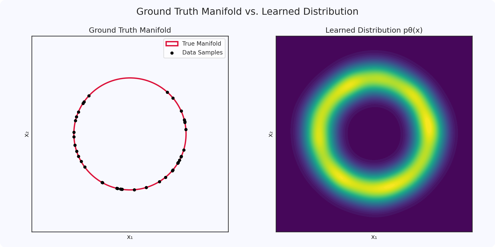
The image on the left shows the ground truth manifold where the data lives. The image on the right shows what our trained model $p_{\theta}$ has learned, a "probability cloud" that correctly identifies the region around the true manifold.

For the mathematically inclined

Formally, we describe the ambient space as $\mathcal X=\mathbb R^{D}$. The data manifold $\mathcal M$ is a compact submanifold with a much smaller intrinsic dimension $d \ll D$. This has a critical consequence: the data occupies zero volume in the larger pixel space, which is why random guessing will never produce a coherent image. Mathematically, this means the true data distribution $p_{\text{data}}$ is singular with respect to the standard volume measure on $\mathbb R^{D}$. Our model's job is to learn a smooth, non-singular distribution that respects this underlying structure.

How do we train such a model?

The classic approach is Maximum Likelihood Estimation (MLE). Given a dataset of real images $\{x_1, x_2, \dots, x_N\}$, we want to adjust our model's parameters $\theta$ (the neural network weights) to maximize the probability, or likelihood, that our model would have generated this data. Mathematically, we maximize the log-likelihood:

$$L(\theta) = \sum \log(p_\theta(x_i))$$

However, we immediately run into a critical problem. Our model doesn't output the final, normalized probabilities $p_\theta(x)$. It outputs an unnormalized score or energy, often written as $p_\theta(x) \propto \exp(-E_\theta(x))$, where $E_\theta(x)$ is an "energy" function learned by the network. To convert this score into a valid probability that integrates to 1, we must divide by the partition function, $Z(\theta)$:

$$p_\theta(x) = \frac{\exp(-E_\theta(x))}{Z(\theta)}, \quad \text{where} \quad Z(\theta) = \int_{\mathbb R^D} \exp(-E_\theta(x')) dx'$$

This integral $Z(\theta)$ represents the total "volume" under the probability surface across the entire high-dimensional space. For our 2D circle example, this is computationally feasible. Now, scale this up to a $512\times 512$ RGB image. The integral is over a $786,432$-dimensional space, a computationally impossible task.

This is the wall that generative modeling research hit. We can define models that produce a score, but we can't turn that score into a proper probability $p_\theta(x)$ to use in our Maximum Likelihood objective function.

Modern approaches like diffusion and flow models are, in essence, highly ingenious methods that provide a "side door" to this problem, allowing us to train expressive distributions without ever calculating the intractable partition function.

Latent Variable Models

Since modeling $p(x)$ directly is too hard, we introduce a "helper", or latent variable, $z$. The core idea is to assume that our complex data $x$ is generated from this simpler, unobserved variable $z$.

• Data ($x$): A final, detailed oil painting of a cat
• Latent Variable ($z$): A simple sketch or a set of high-level instructions: "A fluffy cat, sitting, facing left, looking curious."

We choose the latent space where $z$ lives to be simple, typically a standard multivariate Gaussian distribution $p(z) = \mathcal{N}(0, I)$. This makes it much easier to work with the high-level instructions $z$ than with the millions of individual pixel values $x$.

The Two-Step Generative Process

This reframes generation into two steps:

1. Sample a Latent Code: Draw a simple vector $z$ from the known prior distribution $p(z)$.
2. Decode the Latent Code: Use a powerful neural network, the decoder $p_\theta(x|z)$, to map this simple code $z$ to a complex data point $x$. The marginal probability of an image $x$ is now expressed as an integral over all possible latent codes:

$$p_\theta(x) = \int p_\theta(x|z) p(z) dz$$

This might look like we've just swapped one integral for another, but we've gained a lot. Instead of trying to define a probability distribution over the complex and messy data space directly, we are now learning a mapping from a simple, structured latent space to the complex data manifold.

The New Problem: The Intractable Posterior

We've defined a generative path ($z \rightarrow x$), but how do we train it? To compute the likelihood, we need to evaluate the integral for $p_\theta(x)$. Furthermore, to update our network, we need to know which latent codes $z$ are responsible for a given real image $x$. This requires computing the posterior distribution $p_\theta(z|x)$.Using Bayes' theorem:

$$p_\theta(z|x) = \frac{p_\theta(x|z) p(z)}{p_\theta(x)}$$

Notice our old enemy, the intractable evidence $p_\theta(x)$, is back in the denominator. We are stuck again, unable to infer the latent code for a given image.

The Solution: Variational Autoencoders (VAEs)

This is where variational inference comes in. Since we cannot compute the true posterior $p_\theta(z|x)$, we approximate it, with a second neural network called an encoder or inference network, denoted $q_\phi(z|x)$.

• The Encoder's Job: Takes a real image $x$ and predicts a distribution in the latent space from which $x$ was likely generated. It learns to approximate the true (but intractable) posterior
• The Decoder's Job: Takes a point $z$ from the encoder's predicted distribution and reconstructs the original image $x$

The VAE architecture uses an encoder-decoder framework to learn a generative model of data.

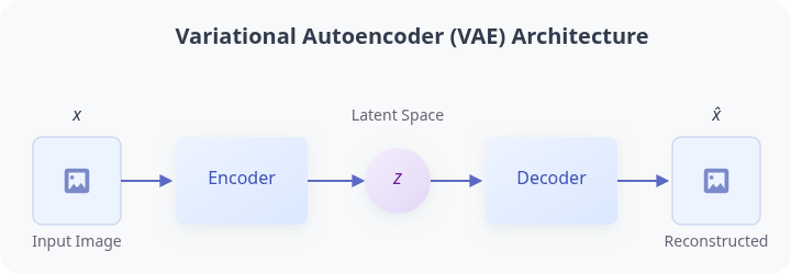
This encoder-decoder framework is trained by maximizing a single, elegant objective function: the Evidence Lower Bound (ELBO). The ELBO cleverly sidesteps the intractable posterior by instead optimizing a lower bound on the true log-likelihood of the data. It balances two competing goals encapsulated in its two terms:

$$\mathcal L(\theta,\phi;x) = \underbrace{\mathbb E_{q_{\phi}(z|x)}\!\left[\log p_{\theta}(x|z)\right]}_\text{Reconstruction Term} - \underbrace{D_{\text{KL}}\!\bigl(q_{\phi}(z|x)\parallel p(z)\bigr)}_\text{Regularization Term}$$

1. The Reconstruction Term pushes the decoder to accurately reconstruct the input image $x$ from its latent code $z$. This ensures the latent code contains meaningful information.
2. The Regularization Term acts as an organizer, forcing the distributions predicted by the encoder $q_\phi(z|x)$ to stay close to the simple prior $p(z)$. This creates a smooth, continuous latent space suitable for generation.

Extension: Controlling Generation with Conditional VAEs

Now that we have the VAE framework, how can we guide the generation process? For instance, how do we ask for an image of a specific object? This is achieved by conditioning the model on extra information $y$ (e.g., a text embedding).

The goal becomes sampling from the conditional distribution $p_\theta(x|y)$. We achieve this by feeding the condition $y$ into both the encoder and the decoder:

• Conditional Encoder: $q_\phi(z|x, y)$ learns to produce a latent code for $x$ given its label $y$
• Conditional Decoder: $p_\theta(x|z, y)$ learns to reconstruct $x$ from its code $z$ while respecting the condition $y$

The marginal probability becomes:

$$p_\theta(x|y) = \int p_\theta(x|z, y) p(z) dz$$

This architecture, known as a Conditional VAE (CVAE), is a foundational principle behind controllable generation and modern text-to-image models.

---

FAQ: Mathematical Foundations of Generative AI

What is the main goal of a generative model?

The primary goal of a generative model is to learn the underlying probability distribution of a given dataset. By doing so, it can create new, synthetic data samples that are statistically similar to the original data.

Why is the partition function a problem in generative modeling?

The partition function is a normalization constant required to turn a model's raw output scores into valid probabilities. It involves an integral over the entire data space, which is computationally intractable for high-dimensional data like images, making it impossible to train models using standard Maximum Likelihood Estimation.

How do latent variable models solve this problem?

Latent variable models circumvent the intractable partition function by introducing a simpler, low-dimensional latent space. Instead of modeling the complex data distribution directly, they learn a mapping from the simple latent space to the complex data space, which is a more manageable task.

What is a Variational Autoencoder (VAE)?

A VAE is a type of generative model that uses an encoder-decoder architecture. The encoder maps input data into a latent distribution, and the decoder reconstructs the data from a sample of that distribution. It's trained to both reconstruct data accurately and keep its latent space well-organized, allowing it to generate new data.